In this article, we’ll present a Mobile Image-to-Image Translation system based on a Cycle-Consistent Adversarial Network (CycleGAN). We’ll build a CycleGAN that can perform unpaired image-to-image translation, as well as show you some entertaining yet academically deep examples. We’ll also discuss how such a trained network, built with TensorFlow and Keras, can be converted to TensorFlow Lite and used as an app on mobile devices.

We assume that you are familiar with the concepts of Deep Learning, as well as with Jupyter Notebooks and TensorFlow. You are welcome to download the project code. In this article, we’ll train and test the network on the horse2zebra dataset and evaluate its performance.

Training CycleGAN

Time to train our CycleGAN to perform some entertaining translations, such as horses to zebras and vice versa. We’ll start by setting a checkpoint path to save the best model:

```checkpoint_path = "./checkpoints/train"

ckpt = tf.train.Checkpoint(generator_g=generator_g, generator_f=generator_f, discriminator_x=discriminator_x, discriminator_y=discriminator_y, generator_g_optimizer=generator_g_optimizer, generator_f_optimizer=generator_f_optimizer, discriminator_x_optimizer=discriminator_x_optimizer, discriminator_y_optimizer=discriminator_y_optimizer)

ckpt_manager = tf.train.CheckpointManager(ckpt, checkpoint_path, max_to_keep=5)

if a checkpoint exists, restore the latest checkpoint

if ckpt_manager.latest_checkpoint: ckpt.restore(ckpt_manager.latest_checkpoint) print ('Latest checkpoint restored!!')

For starters, we’ll train over 20 epochs and see if that is enough for acceptable results. Depending on the obtained results, we might need to increase the number of epochs. Even if your training results appear to be good, prediction may still be less accurate. Hence, 80 to 100 epochs will more likely get you perfect translation, however this will take more than 3 days of training unless you are using a system with very high specifications or paid cloud-based computing services such as AWS or Microsoft Azure.
```EPOCHS = 20
def generate_images(model, test_input):
  prediction = model(test_input)

  plt.figure(figsize=(12, 12))

  display_list = [test_input[0], prediction[0]]
  title = ['Input Image', 'Predicted Image']

  for i in range(2):
    plt.subplot(1, 2, i+1)
    plt.title(title[i])
    # getting the pixel values between [0, 1] to plot it.
    plt.imshow(display_list[i] * 0.5 + 0.5)
    plt.axis('off')
  plt.show()


def train_step(real_x, real_y):
  # persistent is set to True because the tape is used more than
  # once to calculate the gradients.
  with tf.GradientTape(persistent=True) as tape:
    # Generator G translates X -> Y
    # Generator F translates Y -> X.

    fake_y = generator_g(real_x, training=True)
    cycled_x = generator_f(fake_y, training=True)

    fake_x = generator_f(real_y, training=True)
    cycled_y = generator_g(fake_x, training=True)

    # same_x and same_y are used for identity loss.
    same_x = generator_f(real_x, training=True)
    same_y = generator_g(real_y, training=True)

    disc_real_x = discriminator_x(real_x, training=True)
    disc_real_y = discriminator_y(real_y, training=True)

    disc_fake_x = discriminator_x(fake_x, training=True)
    disc_fake_y = discriminator_y(fake_y, training=True)

    # calculate the loss
    gen_g_loss = generator_loss(disc_fake_y)
    gen_f_loss = generator_loss(disc_fake_x)

    total_cycle_loss = calc_cycle_loss(real_x, cycled_x) + calc_cycle_loss(real_y, cycled_y)

    # Total generator loss = adversarial loss + cycle loss
    total_gen_g_loss = gen_g_loss + total_cycle_loss + identity_loss(real_y, same_y)
    total_gen_f_loss = gen_f_loss + total_cycle_loss + identity_loss(real_x, same_x)

    disc_x_loss = discriminator_loss(disc_real_x, disc_fake_x)
    disc_y_loss = discriminator_loss(disc_real_y, disc_fake_y)

  # Calculate the gradients for generator and discriminator
  generator_g_gradients = tape.gradient(total_gen_g_loss, 
                                        generator_g.trainable_variables)
  generator_f_gradients = tape.gradient(total_gen_f_loss, 
                                        generator_f.trainable_variables)

  discriminator_x_gradients = tape.gradient(disc_x_loss, 
                                            discriminator_x.trainable_variables)
  discriminator_y_gradients = tape.gradient(disc_y_loss, 
                                            discriminator_y.trainable_variables)

  # Apply the gradients to the optimizer
  generator_g_optimizer.apply_gradients(zip(generator_g_gradients, 
                                            generator_g.trainable_variables))

  generator_f_optimizer.apply_gradients(zip(generator_f_gradients, 
                                            generator_f.trainable_variables))

  discriminator_x_optimizer.apply_gradients(zip(discriminator_x_gradients,
                                                discriminator_x.trainable_variables))

  discriminator_y_optimizer.apply_gradients(zip(discriminator_y_gradients,
                                                discriminator_y.trainable_variables))

The training loop above does the following:

• Gets predictions
• Calculates the loss
• Calculates the gradients using backpropagation

• Applies the gradients to the optimizerDuring the training, the network will select a random image from the training set and display it along with its translated version to let us visualize how the performance changes after every epoch, as shown in the figure below. for epoch in range(EPOCHS): start = time.time()

  n = 0 for image_x, image_y in tf.data.Dataset.zip((train_horses, train_zebras)): train_step(image_x, image_y) if n % 10 == 0:

  print ('.', end='')
  

  n += 1

  clear_output(wait=True)

  Using a consistent image (sample_horse) so that the progress of the model

  is clearly visible.

  generate_images(generator_g, sample_horse)

  if (epoch + 1) % 5 == 0: ckpt_save_path = ckpt_manager.save() print ('Saving checkpoint for epoch {} at {}'.format(epoch+1,

                                                     ckpt_save_path))
  

  print ('Time taken for epoch {} is {} sec\n'.format(epoch + 1,

                                                  time.time()-start))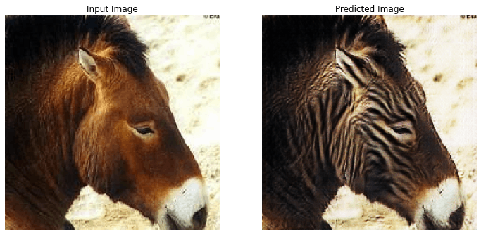
  

  

**Evaluating CycleGAN

** Once the CycleGAN has been trained, we can start feeding it new images and evaluating its performance in translating horses to zebras and vice versa.

Let’s test our trained CycleGAN on images from the dataset and visualize its generalization power. We’ll use the generate_images function, which will pick up some images, pass them through the trained network, and display the translation results.

```def generate_images(model, test_input): prediction = model(test_input)

plt.figure(figsize=(12, 12))

display_list = [test_input[0], prediction[0]] title = ['Input Image', 'Predicted Image']

for i in range(2): plt.subplot(1, 2, i+1) plt.title(title[i])

# getting the pixel values between [0, 1] to plot it.
plt.imshow(display_list[i] * 0.5 + 0.5)
plt.axis('off')

plt.show()

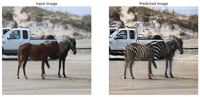
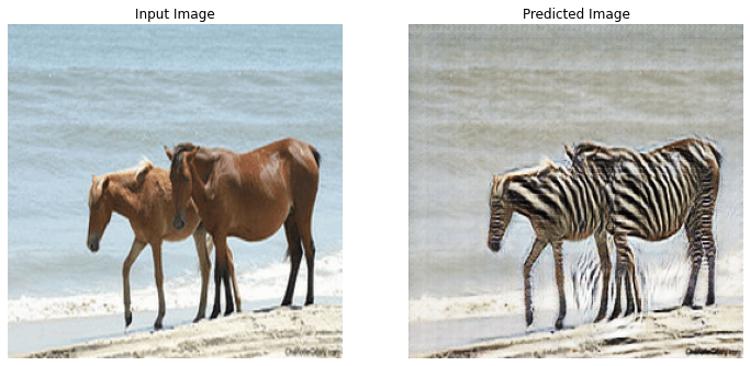
Now, you can choose any test image and visualize the translation result:



```for inp in test_horses.take(5):
  generate_images(generator_g, inp)

Here are some examples obtained after the network had been trained over only 20 epochs. The results are quite good for such a short training. You can improve them by adding more epochs.

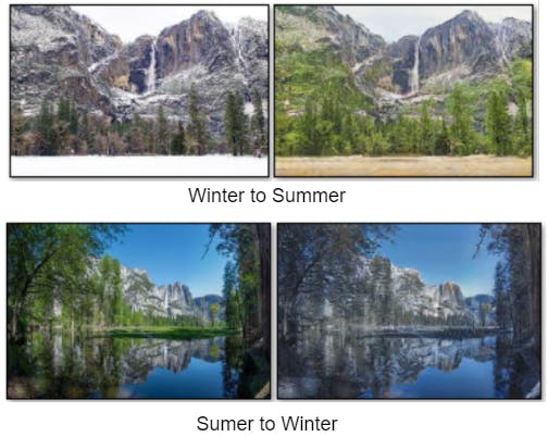
**Season Transfer CycleGAN

** We can use the network we’ve designed for different tasks, such as day to night transfer or season transfer. In order to train our network for season transfer, all we need to do is change the training dataset to summer2winter.

We trained our network on the above dataset for 80 epochs. Have a look at the results.

P.s. the whole source code is available on my github